1. 输入输出

训练输入： \[ X= \{x_1, x_2, ..., x_N\} \\ Z=\{z_1,z_2,...,z_{N}\} \] 其中，

$x_i \in \mathbb{R}^{m},i =1,2,...,N$，$x_i$ 为特征域
$z_i \in \mathbb{R}^k,,i =1,2,...,N$，$z_i$ 为噪声域

测试输入 \[ Z'=\{z'_1,z'_2,...,z'_{N'}\},z'_i \in \mathbb{R}^k \] 测试输出： \[ \hat X'=\{\hat x'_1, \hat x'_2,..., \hat x'_{N'}\},\hat x'_i \in \mathbb{R}^m \]

2. 基本定义

2.1. 模型推导

这是一张目前各类生成模型框架的对比图

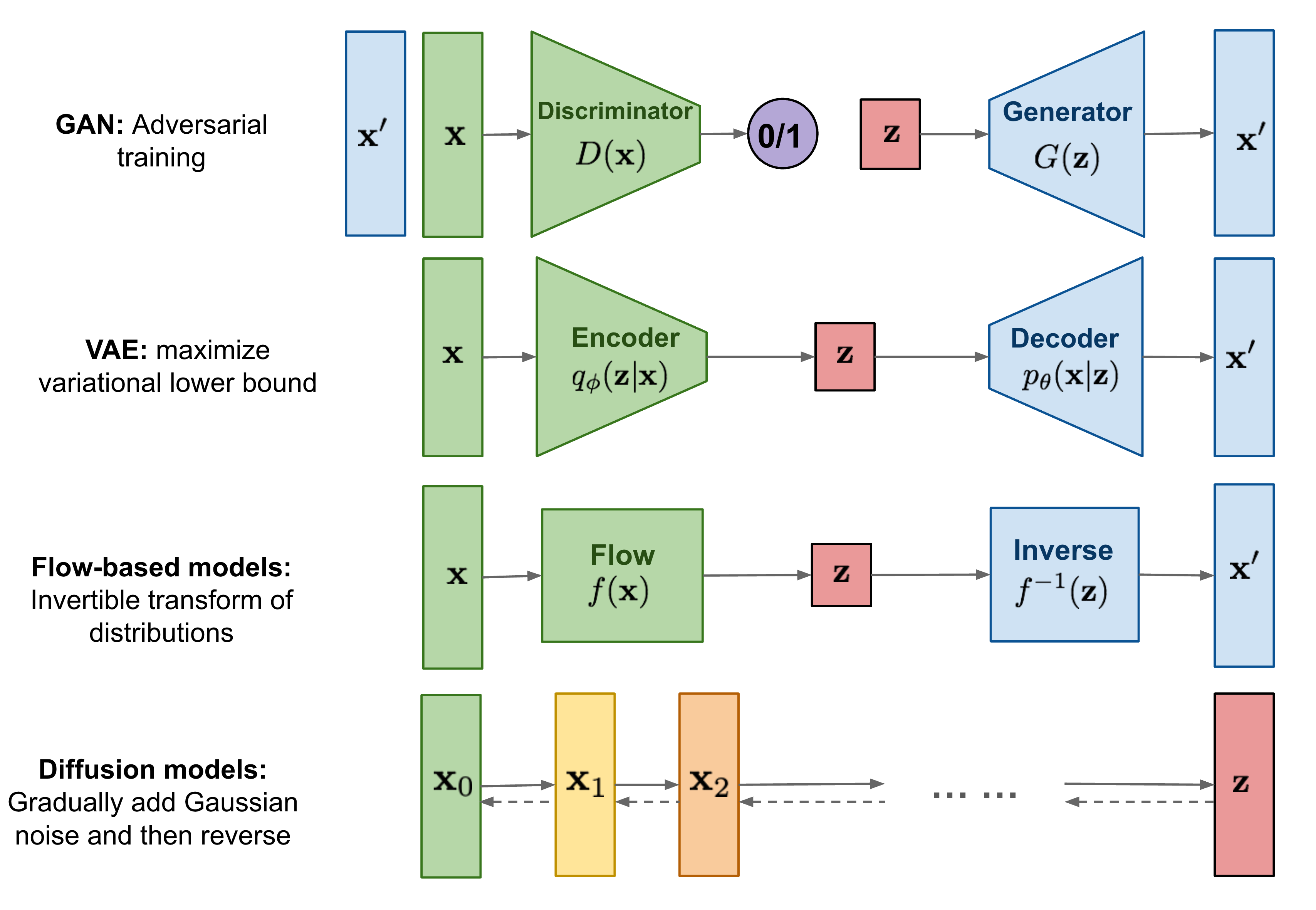
Diffusion Model的思想很简单：对数据域 $\mathbf x$ 不断添加高斯噪声，且保持每一时刻的分布仍为高斯分布，最终变换至噪声域 $\mathbf z$ ；然后再将噪声域 $\mathbf z$ 再逐步还原回数据域 $\mathbf x$

2.2. 学习策略

首先来推导添加噪声的过程

首先推导 $\mathbf x_t$ 关于 $\mathbf x_{t-1}$ 的表达形式（其实这一步不需要怎么推导，因为大部分的结论都是直接假设出来的）

不妨设

$\mathbf x_0 \sim q(\mathbf x_0),\mathbf x_t = q(\mathbf{x}_t \vert \mathbf{x}_{t-1})$
每一个时刻 $t-1$ 往前叠加高斯噪声 $\mathcal{N}(\mathbf{x}_t; \sqrt{1 - \beta_t} \mathbf{x}_{t-1}, \beta_t\mathbf{I})$，其中，$\beta_t \in (0, 1)$ 是关于噪声集的超参数，一般是一个随 $t$ 单调递增的线性函数。
$\mathbf x_t$ 只与 $\mathbf x_{t-1}$ 有关

则有 \[ q(\mathbf{x}_t \vert \mathbf{x}_{t-1}) = \mathcal{N}(\mathbf{x}_t; \sqrt{1 - \beta_t} \mathbf{x}_{t-1}, \beta_t\mathbf{I}) \\ q(\mathbf{x}_{1:T} \vert \mathbf{x}_0) = \prod^T_{t=1} q(\mathbf{x}_t \vert \mathbf{x}_{t-1}) \] 然后再推导 $\mathbf x_t$ 关于 $\mathbf x_0$ 的表达形式（这一步推导的目的是方便后续的反向推导）

不妨再设

$\alpha_t = 1 - \beta_t, \bar{\alpha}_t = \prod_{i=1}^t \alpha_i$
$\boldsymbol{\epsilon}_t \sim \mathcal{N}(\mathbf{0}, \mathbf{I}), \bar{\boldsymbol{\epsilon}}_t \sim \mathcal{N}(\mathbf{0}, \mathbf{I})$，其中，$\{ \boldsymbol{\epsilon}_t \}$ 集合内均为相互独立的分布， $\bar{\boldsymbol{\epsilon}}_i$ 是 $\{ \boldsymbol{\epsilon}_{T-i}| i=1,2,\cdots T \}$ 集合内所有的分布的叠加分布

则有 \[ \begin{aligned} \mathbf{x}_t &= \sqrt{\alpha_t}\mathbf{x}_{t-1} + \sqrt{1 - \alpha_t}\boldsymbol{\epsilon}_{t-1} \\ &= \sqrt{\alpha_t} (\sqrt{\alpha_{t-1}}\mathbf{x}_{t-2} + \sqrt{1 - \alpha_{t-1}}\boldsymbol{\epsilon}_{t-2}) + \sqrt{1 - \alpha_t}\boldsymbol{\epsilon}_{t-1} \\ &= \sqrt{\alpha_t \alpha_{t-1}} \mathbf{x}_{t-2} + \sqrt{1 - \alpha_t \alpha_{t-1}} \bar{\boldsymbol{\epsilon}}_{2} \\ &= \dots \\ &= \sqrt{\bar{\alpha}_t}\mathbf{x}_0 + \sqrt{1 - \bar{\alpha}_t}\bar{\boldsymbol{\epsilon}}_t \\ q(\mathbf{x}_t \vert \mathbf{x}_0) &= \mathcal{N}(\mathbf{x}_t; \sqrt{\bar{\alpha}_t} \mathbf{x}_0, (1 - \bar{\alpha}_t)\mathbf{I}) \end{aligned} \]

注：

上面推导中，

第一步应用了重参数技巧，该技巧已经在VAE中提及过，这里就不再赘述了

第三步应用了独立高斯分布可加性 $\mathcal{N}(\mathbf{0}, \sigma_1^2\mathbf{I}) + \mathcal{N}(\mathbf{0}, \sigma_2^2\mathbf{I}) = \mathcal{N}(\mathbf{0}, (\sigma_1^2 + \sigma_2^2)\mathbf{I})$，即可推导出 $\sqrt{(1 - \alpha_t)}\boldsymbol{\epsilon}_{t-1} + \sqrt {\alpha_t (1-\alpha_{t-1})} \boldsymbol{\epsilon}_{t-2} = \sqrt{1 - \alpha_t\alpha_{t-1}} \bar{\boldsymbol{\epsilon}}_{2}$

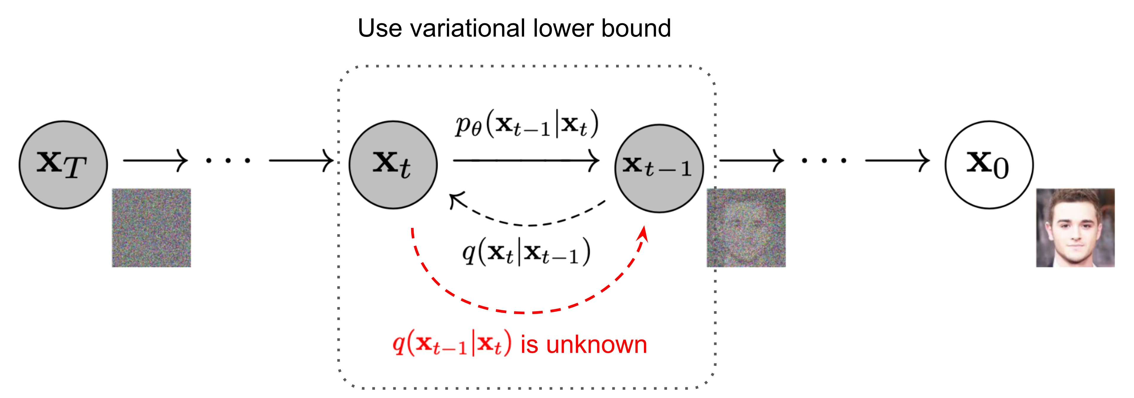
下面来看消除噪声的过程，这一部分的目的是还原 $q(\mathbf{x}_{t-1} \vert \mathbf{x}_{t})$ 表达形式

$q(\mathbf{x}_{t-1} \vert \mathbf{x}_{t})$ 未知且不可求，但可以证明，当 $q(\mathbf{x}_t \vert \mathbf{x}_{t-1})$ 满足高斯分布，且 $\beta_t$ 较小时，$q(\mathbf{x}_{t-1} \vert \mathbf{x}_{t})$ 仍满足高斯分布。所以模型的还原问题可以转化为，每一个时刻向前叠加一个高斯分布，使其还原为原来的分布

注：

这一部分仍然属于前向推导，尽管从上面模型图中看起来的是属于反向推导，但实际上，上面的模型图是做了折叠处理，将模型图展开便可以得到一个类似于编码-解码的对称结构，加噪是编码，降噪是解码

由于加噪过程不存在未知变量，所以实际模型构建的时候只有降噪部分结构，即输入 $\mathbf x_T = \mathbf z$，输出 $\mathbf x_0 \sim q(\mathbf x_0)$

不妨设

$\mathbf x_t \sim p_\theta(\mathbf x),\mathbf x_{t-1} = p_\theta(\mathbf{x}_{t-1} \vert \mathbf{x}_t)$
每一个时刻 $t$ 往后叠加高斯噪声 $\mathcal{N}(\mathbf{x}_{t-1}; \boldsymbol{\mu}_\theta(\mathbf{x}_t, t), \boldsymbol{\Sigma}_\theta(\mathbf{x}_t, t))$

则有 \[ p_\theta(\mathbf{x}_{0:T}) = p(\mathbf{x}_T) \prod^T_{t=1} p_\theta(\mathbf{x}_{t-1} \vert \mathbf{x}_t) \\ p_\theta(\mathbf{x}_{t-1} \vert \mathbf{x}_t) = \mathcal{N}(\mathbf{x}_{t-1}; \boldsymbol{\mu}_\theta(\mathbf{x}_t, t), \boldsymbol{\Sigma}_\theta(\mathbf{x}_t, t)) \] 但上式中的参数 $\boldsymbol{\mu}_\theta(\mathbf{x}_t, t), \boldsymbol{\Sigma}_\theta(\mathbf{x}_t, t)$ 没有办法直接求解，所以使用万能的神经网络进行拟合。

由于 $q(\mathbf{x}_{t-1} \vert \mathbf{x}_{t})$ 不能直接获得，所以 $p_\theta(\mathbf{x}_{t-1} \vert \mathbf{x}_t)$ 不能直接拟合 $q(\mathbf{x}_{t-1} \vert \mathbf{x}_{t})$ ，暂时没什么好的思路。

这里不妨先跳到模型损失函数的推导。

2.3. 学习算法

模型的目的是比较真实样本和生成样本的差距，所以选择优化 $q(\mathbf x_0)$ 和 $p_{\theta}(\mathbf x_0)$ 的交叉熵 \[ L=\mathbb{E}_{q\left(x_0\right)}\left[-\log p_\theta\left(x_0\right)\right] \] 但 $p_\theta\left(x_0\right)$ 目前还是未知的，但可以通过变分下限（VLB）的方法，巧妙地消去 \[ \begin{aligned} - \log p_\theta(\mathbf{x}_0) &\leq - \log p_\theta(\mathbf{x}_0) + D_\text{KL}(q(\mathbf{x}_{1:T}\vert\mathbf{x}_0) \| p_\theta(\mathbf{x}_{1:T}\vert\mathbf{x}_0) ) \\ &= -\log p_\theta(\mathbf{x}_0) + \mathbb{E}_{\mathbf{x}_{1:T}\sim q(\mathbf{x}_{1:T} \vert \mathbf{x}_0)} \Big[ \log\frac{q(\mathbf{x}_{1:T}\vert\mathbf{x}_0)}{p_\theta(\mathbf{x}_{0:T}) / p_\theta(\mathbf{x}_0)} \Big] \\ &= -\log p_\theta(\mathbf{x}_0) + \mathbb{E}_q \Big[ \log\frac{q(\mathbf{x}_{1:T}\vert\mathbf{x}_0)}{p_\theta(\mathbf{x}_{0:T})} + \log p_\theta(\mathbf{x}_0) \Big] \\ &= \mathbb{E}_q \Big[ \log \frac{q(\mathbf{x}_{1:T}\vert\mathbf{x}_0)}{p_\theta(\mathbf{x}_{0:T})} \Big] \end{aligned} \] 代入上式中，应用fubini定理，有 \[ \begin{aligned} L_\text{VLB} &=\mathbb{E}_{q\left(x_0\right)}\left(\mathbb{E}_{q\left(x_{1-T} \mid x_0\right)}\left[\log \frac{q\left(x_{1 ; T} \mid x_0\right)}{p_\theta\left(x_{0: T}\right)}\right]\right) \\ &= \mathbb{E}_{q(\mathbf{x}_{0:T})} \Big[ \log \frac{q(\mathbf{x}_{1:T}\vert\mathbf{x}_0)}{p_\theta(\mathbf{x}_{0:T})} \Big] \\ &\geq - \mathbb{E}_{q(\mathbf{x}_0)} \log p_\theta(\mathbf{x}_0) \end{aligned} \]

注：

上式也可以通过Jensen不等式推导得出 \[ \begin{aligned} L &= - \mathbb{E}_{q(\mathbf{x}_0)} \log p_\theta(\mathbf{x}_0) \\ &= - \mathbb{E}_{q(\mathbf{x}_0)} \log \Big( \int p_\theta(\mathbf{x}_{0:T}) d\mathbf{x}_{1:T} \Big) \\ &= - \mathbb{E}_{q(\mathbf{x}_0)} \log \Big( \int q(\mathbf{x}_{1:T} \vert \mathbf{x}_0) \frac{p_\theta(\mathbf{x}_{0:T})}{q(\mathbf{x}_{1:T} \vert \mathbf{x}_{0})} d\mathbf{x}_{1:T} \Big) \\ &= - \mathbb{E}_{q(\mathbf{x}_0)} \log \Big( \mathbb{E}_{q(\mathbf{x}_{1:T} \vert \mathbf{x}_0)} \frac{p_\theta(\mathbf{x}_{0:T})}{q(\mathbf{x}_{1:T} \vert \mathbf{x}_{0})} \Big) \\ &\leq - \mathbb{E}_{q(\mathbf{x}_{0:T})} \log \frac{p_\theta(\mathbf{x}_{0:T})}{q(\mathbf{x}_{1:T} \vert \mathbf{x}_{0})} \\ &= \mathbb{E}_{q(\mathbf{x}_{0:T})}\Big[\log \frac{q(\mathbf{x}_{1:T} \vert \mathbf{x}_{0})}{p_\theta(\mathbf{x}_{0:T})} \Big] = L_\text{VLB} \end{aligned} \] 上面过程的第五步即应用了Jensen不等式

对 $L_\text{VLB}$ 进一步展开 \[ \begin{aligned} L_\text{VLB} &= \mathbb{E}_{q(\mathbf{x}_{0:T})} \Big[ \log\frac{q(\mathbf{x}_{1:T}\vert\mathbf{x}_0)}{p_\theta(\mathbf{x}_{0:T})} \Big] \\ &= \mathbb{E}_q \Big[ \log\frac{\prod_{t=1}^T q(\mathbf{x}_t\vert\mathbf{x}_{t-1})}{ p_\theta(\mathbf{x}_T) \prod_{t=1}^T p_\theta(\mathbf{x}_{t-1} \vert\mathbf{x}_t) } \Big] \\ &= \mathbb{E}_q \Big[ -\log p_\theta(\mathbf{x}_T) + \sum_{t=1}^T \log \frac{q(\mathbf{x}_t\vert\mathbf{x}_{t-1})}{p_\theta(\mathbf{x}_{t-1} \vert\mathbf{x}_t)} \Big] \\ &= \mathbb{E}_q \Big[ -\log p_\theta(\mathbf{x}_T) + \sum_{t=2}^T \log \frac{q(\mathbf{x}_t\vert\mathbf{x}_{t-1})}{p_\theta(\mathbf{x}_{t-1} \vert\mathbf{x}_t)} + \log\frac{q(\mathbf{x}_1 \vert \mathbf{x}_0)}{p_\theta(\mathbf{x}_0 \vert \mathbf{x}_1)} \Big] \\ &= \mathbb{E}_q \Big[ -\log p_\theta(\mathbf{x}_T) + \sum_{t=2}^T \log \Big( \frac{q(\mathbf{x}_{t-1} \vert \mathbf{x}_t, \mathbf{x}_0)}{p_\theta(\mathbf{x}_{t-1} \vert\mathbf{x}_t)}\cdot \frac{q(\mathbf{x}_t \vert \mathbf{x}_0)}{q(\mathbf{x}_{t-1}\vert\mathbf{x}_0)} \Big) + \log \frac{q(\mathbf{x}_1 \vert \mathbf{x}_0)}{p_\theta(\mathbf{x}_0 \vert \mathbf{x}_1)} \Big] \\ &= \mathbb{E}_q \Big[ -\log p_\theta(\mathbf{x}_T) + \sum_{t=2}^T \log \frac{q(\mathbf{x}_{t-1} \vert \mathbf{x}_t, \mathbf{x}_0)}{p_\theta(\mathbf{x}_{t-1} \vert\mathbf{x}_t)} + \sum_{t=2}^T \log \frac{q(\mathbf{x}_t \vert \mathbf{x}_0)}{q(\mathbf{x}_{t-1} \vert \mathbf{x}_0)} + \log\frac{q(\mathbf{x}_1 \vert \mathbf{x}_0)}{p_\theta(\mathbf{x}_0 \vert \mathbf{x}_1)} \Big] \\ &= \mathbb{E}_q \Big[ -\log p_\theta(\mathbf{x}_T) + \sum_{t=2}^T \log \frac{q(\mathbf{x}_{t-1} \vert \mathbf{x}_t, \mathbf{x}_0)}{p_\theta(\mathbf{x}_{t-1} \vert\mathbf{x}_t)} + \log\frac{q(\mathbf{x}_T \vert \mathbf{x}_0)}{q(\mathbf{x}_1 \vert \mathbf{x}_0)} + \log \frac{q(\mathbf{x}_1 \vert \mathbf{x}_0)}{p_\theta(\mathbf{x}_0 \vert \mathbf{x}_1)} \Big]\\ &= \mathbb{E}_q \Big[ \log\frac{q(\mathbf{x}_T \vert \mathbf{x}_0)}{p_\theta(\mathbf{x}_T)} + \sum_{t=2}^T \log \frac{q(\mathbf{x}_{t-1} \vert \mathbf{x}_t, \mathbf{x}_0)}{p_\theta(\mathbf{x}_{t-1} \vert\mathbf{x}_t)} - \log p_\theta(\mathbf{x}_0 \vert \mathbf{x}_1) \Big] \\ &= \mathbb{E}_q [\underbrace{D_\text{KL}(q(\mathbf{x}_T \vert \mathbf{x}_0) \parallel p_\theta(\mathbf{x}_T))}_{L_T} + \sum_{t=2}^T \underbrace{D_\text{KL}(q(\mathbf{x}_{t-1} \vert \mathbf{x}_t, \mathbf{x}_0) \parallel p_\theta(\mathbf{x}_{t-1} \vert\mathbf{x}_t))}_{L_{t-1}} \underbrace{- \log p_\theta(\mathbf{x}_0 \vert \mathbf{x}_1)}_{L_0} ] \\ &= L_T + L_{T-1} + \dots + L_0 \end{aligned} \] 其中，由于$q(\mathbf{x}_T \vert \mathbf{x}_0)$ 没有未知变量，所以 $L_T$ 可忽略；而 $L_0$ 用了一种名为separate discrete decoder的处理手段，将 $L_0$ 处理成一般常量忽略。

所以上式只需关注 $L_t$ 即可。这里书接上一回，回到之前的前向推导，$p_\theta(\mathbf{x}_{t-1} \vert \mathbf{x}_t)$ 可以拟合 $q(\mathbf{x}_t \vert \mathbf{x}_{t-1}, \mathbf{x}_0)$

问题转化为对 $q(\mathbf{x}_t \vert \mathbf{x}_{t-1}, \mathbf{x}_0)$ 的推导，根据贝叶斯定理，可得 \[ \begin{aligned} q(\mathbf{x}_{t-1} \vert \mathbf{x}_t, \mathbf{x}_0) &= q(\mathbf{x}_t \vert \mathbf{x}_{t-1}, \mathbf{x}_0) \frac{ q(\mathbf{x}_{t-1} \vert \mathbf{x}_0) }{ q(\mathbf{x}_t \vert \mathbf{x}_0) } \\ &\propto \exp \Big(-\frac{1}{2} \big(\frac{(\mathbf{x}_t - \sqrt{\alpha_t} \mathbf{x}_{t-1})^2}{\beta_t} + \frac{(\mathbf{x}_{t-1} - \sqrt{\bar{\alpha}_{t-1}} \mathbf{x}_0)^2}{1-\bar{\alpha}_{t-1}} - \frac{(\mathbf{x}_t - \sqrt{\bar{\alpha}_t} \mathbf{x}_0)^2}{1-\bar{\alpha}_t} \big) \Big) \\ &= \exp \Big(-\frac{1}{2} \big(\frac{\mathbf{x}_t^2 - 2\sqrt{\alpha_t} \mathbf{x}_t \color{blue}{\mathbf{x}_{t-1}} \color{black}{+ \alpha_t} \color{red}{\mathbf{x}_{t-1}^2} }{\beta_t} + \frac{ \color{red}{\mathbf{x}_{t-1}^2} \color{black}{- 2 \sqrt{\bar{\alpha}_{t-1}} \mathbf{x}_0} \color{blue}{\mathbf{x}_{t-1}} \color{black}{+ \bar{\alpha}_{t-1} \mathbf{x}_0^2} }{1-\bar{\alpha}_{t-1}} - \frac{(\mathbf{x}_t - \sqrt{\bar{\alpha}_t} \mathbf{x}_0)^2}{1-\bar{\alpha}_t} \big) \Big) \\ &= \exp\Big( -\frac{1}{2} \big( \color{red}{(\frac{\alpha_t}{\beta_t} + \frac{1}{1 - \bar{\alpha}_{t-1}})} \mathbf{x}_{t-1}^2 - \color{blue}{(\frac{2\sqrt{\alpha_t}}{\beta_t} \mathbf{x}_t + \frac{2\sqrt{\bar{\alpha}_{t-1}}}{1 - \bar{\alpha}_{t-1}} \mathbf{x}_0)} \mathbf{x}_{t-1} \color{black}{ + C(\mathbf{x}_t, \mathbf{x}_0) \big) \Big)} \\ &\propto \mathcal{N}(\mathbf{x}_{t-1}; \color{blue}{\tilde{\boldsymbol{\mu}}}(\mathbf{x}_t, \mathbf{x}_0), \color{red}{\tilde{\beta}_t} \mathbf{I}) \end{aligned} \]

注：

第二步和第四步中，应用了变换 $\mathcal{N}(\mu, \sigma^2) = \exp \left(-\frac{(x-\mu)^2}{2 \sigma^2}\right)=\exp \left(-\frac{1}{2}\left(\frac{1}{\sigma^2} x^2-\frac{2 \mu}{\sigma^2} x+\frac{\mu^2}{\sigma^2}\right)\right)$

可得 \[ \begin{aligned} \tilde{\beta}_t &= 1/(\frac{\alpha_t}{\beta_t} + \frac{1}{1 - \bar{\alpha}_{t-1}}) \\ &= 1/(\frac{\alpha_t - \bar{\alpha}_t + \beta_t}{\beta_t(1 - \bar{\alpha}_{t-1})}) \\ &= {\frac{1 - \bar{\alpha}_{t-1}}{1 - \bar{\alpha}_t} \cdot \beta_t} \\ \tilde{\boldsymbol{\mu}}_t (\mathbf{x}_t, \mathbf{x}_0) &= (\frac{\sqrt{\alpha_t}}{\beta_t} \mathbf{x}_t + \frac{\sqrt{\bar{\alpha}_{t-1} }}{1 - \bar{\alpha}_{t-1}} \mathbf{x}_0)/(\frac{\alpha_t}{\beta_t} + \frac{1}{1 - \bar{\alpha}_{t-1}}) \\ &= (\frac{\sqrt{\alpha_t}}{\beta_t} \mathbf{x}_t + \frac{\sqrt{\bar{\alpha}_{t-1} }}{1 - \bar{\alpha}_{t-1}} \mathbf{x}_0) {\frac{1 - \bar{\alpha}_{t-1}}{1 - \bar{\alpha}_t} \cdot \beta_t} \\ &= \frac{\sqrt{\alpha_t}(1 - \bar{\alpha}_{t-1})}{1 - \bar{\alpha}_t} \mathbf{x}_t + \frac{\sqrt{\bar{\alpha}_{t-1}}\beta_t}{1 - \bar{\alpha}_t} \mathbf{x}_0\\ \end{aligned} \] 又从前面 $\mathbf{x}_t$ 的表达式变换可得 \[ \mathbf{x}_0 = \frac{1}{\sqrt{\bar{\alpha}_t}}(\mathbf{x}_t - \sqrt{1 - \bar{\alpha}_t} \bar{\boldsymbol{\epsilon}}_t) \] 代入上式可得 \[ \begin{aligned} \tilde{\boldsymbol{\mu}}_t &= \frac{\sqrt{\alpha_t}(1 - \bar{\alpha}_{t-1})}{1 - \bar{\alpha}_t} \mathbf{x}_t + \frac{\sqrt{\bar{\alpha}_{t-1}}\beta_t}{1 - \bar{\alpha}_t} \frac{1}{\sqrt{\bar{\alpha}_t}}(\mathbf{x}_t - \sqrt{1 - \bar{\alpha}_t}\bar{\boldsymbol{\epsilon}}_t) \\ &= {\frac{1}{\sqrt{\alpha_t}} \Big( \mathbf{x}_t - \frac{1 - \alpha_t}{\sqrt{1 - \bar{\alpha}_t}} \bar{\boldsymbol{\epsilon}}_t \Big)} \end{aligned} \] $p_\theta(\mathbf{x}_{t-1} \vert \mathbf{x}_t)$ 应和 $q(\mathbf{x}_t \vert \mathbf{x}_{t-1}, \mathbf{x}_0)$ 有相似的表达形式，故使用 $\boldsymbol{\epsilon}_\theta(\mathbf{x}_t, t)$ 替换 $\bar{\boldsymbol{\epsilon}}_t$，可得 \[ \boldsymbol{\mu}_\theta(\mathbf{x}_t, t) \propto {\frac{1}{\sqrt{\alpha_t}} \Big( \mathbf{x}_t - \frac{1 - \alpha_t}{\sqrt{1 - \bar{\alpha}_t}} \boldsymbol{\epsilon}_\theta(\mathbf{x}_t, t) \Big)} \\ \sigma_t^2 = \boldsymbol{\Sigma}_\theta(\mathbf{x}_t, t) \propto {\frac{1 - \bar{\alpha}_{t-1}}{1 - \bar{\alpha}_t} \cdot \beta_t} \] 往$\mathbf{x}_t$ 加入$N(0,I)$ 噪声即可得到 $\mathbf{x}_{t-1}$ \[ \mathbf{x}_{t-1} = \boldsymbol{\mu}_\theta(\mathbf{x}_t, t) + \sigma_t z_t \] 其中，$z_t \sim N(0,I)$

于是，根据多元高斯分布的KL散度求解，可对 $L_t$ 进一步展开 \[ \begin{aligned} L_t &= \mathbb{E}_{\mathbf{x}_0, \bar{\boldsymbol{\epsilon}}} \Big[\frac{1}{2 \| \boldsymbol{\Sigma}_\theta(\mathbf{x}_t, t) \|^2_2} \| \color{blue}{\tilde{\boldsymbol{\mu}}_t(\mathbf{x}_t, \mathbf{x}_0)} - \color{green}{\boldsymbol{\mu}_\theta(\mathbf{x}_t, t)} \|^2 \Big] \\ &= \mathbb{E}_{\mathbf{x}_0, \bar{\boldsymbol{\epsilon}}} \Big[\frac{1}{2 \|\boldsymbol{\Sigma}_\theta \|^2_2} \| \color{blue}{\frac{1}{\sqrt{\alpha_t}} \Big( \mathbf{x}_t - \frac{1 - \alpha_t}{\sqrt{1 - \bar{\alpha}_t}} \bar{\boldsymbol{\epsilon}}_t \Big)} - \color{green}{\frac{1}{\sqrt{\alpha_t}} \Big( \mathbf{x}_t - \frac{1 - \alpha_t}{\sqrt{1 - \bar{\alpha}_t}} \boldsymbol{\boldsymbol{\epsilon}}_\theta(\mathbf{x}_t, t) \Big)} \|^2 \Big] \\ &= \mathbb{E}_{\mathbf{x}_0, \bar{\boldsymbol{\epsilon}}} \Big[\frac{ (1 - \alpha_t)^2 }{2 \alpha_t (1 - \bar{\alpha}_t) \| \boldsymbol{\Sigma}_\theta \|^2_2} \|\bar{\boldsymbol{\epsilon}}_t - \boldsymbol{\epsilon}_\theta(\mathbf{x}_t, t)\|^2 \Big] \\ &= \mathbb{E}_{\mathbf{x}_0, \bar{\boldsymbol{\epsilon}}} \Big[\frac{ (1 - \alpha_t)^2 }{2 \alpha_t (1 - \bar{\alpha}_t) \| \boldsymbol{\Sigma}_\theta \|^2_2} \bar{\boldsymbol{\epsilon}}_t - \boldsymbol{\epsilon}_\theta(\sqrt{\bar{\alpha}_t}\mathbf{x}_0 + \sqrt{1 - \bar{\alpha}_t}\bar{\boldsymbol{\epsilon}}_t, t)\|^2 \Big] \end{aligned} \] 最后，论文中发现 $\boldsymbol{\Sigma}_\theta$ 这一项的系数可能会导致训练不稳定，故忽略 $\boldsymbol{\Sigma}_\theta$ 这一项的系数，可进一步化简为 \[ \begin{aligned} L_t^\text{simple} &= \mathbb{E}_{t \sim [1, T], \mathbf{x}_0, \bar{\boldsymbol{\epsilon}}_t} \Big[\| \bar{\boldsymbol{\epsilon}}_t - \boldsymbol{\epsilon}_\theta(\mathbf{x}_t, t)\|^2 \Big] \\ &= \mathbb{E}_{t \sim [1, T], \mathbf{x}_0, \bar{\boldsymbol{\epsilon}}_t} \Big[\| \bar{\boldsymbol{\epsilon}}_t - \boldsymbol{\epsilon}_\theta(\sqrt{\bar{\alpha}_t}\mathbf{x}_0 + \sqrt{1 - \bar{\alpha}_t} \bar{\boldsymbol{\epsilon}}_t, t)\|^2 \Big] \end{aligned} \]

3. 代码实现

训练及推理的伪代码如下

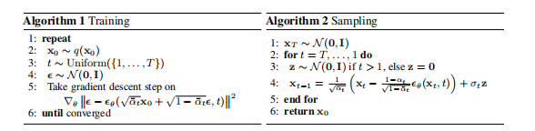
在具体的代码实现中，拟合模型采用Unet结构，输入为 $_{t} $，输出 $\mathbf{h}_{t}$ 则可以选择拟合以下三种变量

$\mathbf{h}_{t}=\boldsymbol{\epsilon}_t$，则 \[ \mathbf{x}_{t-1} = \tilde{\boldsymbol{\mu}}_t (\mathbf{x}_t, \mathbf{x}_0) + \sigma_t z_t \\ L_t^\text{simple}=\mathbb{E}_{t \sim [1, T], \mathbf{x}_0, \bar{\boldsymbol{\epsilon}}_t} \Big[\| \bar{\boldsymbol{\epsilon}}_t - \boldsymbol{\epsilon}_t\|^2 \Big] \] 其中，$\sigma_t= e ^ {0.5 \log \sigma_t^2}$（注：其实这里不太理解为什么不直接用 $\sigma_t=\sqrt{\sigma_t^2}$ ），$\bar{\boldsymbol{\epsilon}}_t$ 是随机生成的高斯分布噪声
$\mathbf{h}_{t}=\mathbf{x}_{0}$，则 \[ \mathbf{x}_{t-1} = \tilde{\boldsymbol{\mu}}_t (\mathbf{x}_t, \mathbf{x}_0) + \sigma_t z_t \\ L_t^\text{simple}=\mathbb{E}_{t \sim [1, T], \mathbf{x}_0, \bar{\boldsymbol{\epsilon}}_t} \Big[\| \bar{\mathbf{x}}_0 - \mathbf{x}_{0}\|^2 \Big] \] 其中，$\bar{\mathbf{x}}_0$ 为真实的图片输入
$\mathbf{h}_{t} = \mathbf{v}_{t}$，令 $\mathbf{v}_{t} = \sqrt{\bar{\alpha}_t} z_t - \sqrt{1 - \bar{\alpha}_t}\mathbf{x}_0$，则 \[ \mathbf{x}_{t-1} = \tilde{\boldsymbol{\mu}}_t (\mathbf{x}_t, \mathbf{x}_0) + \sigma_t z_t \\ L_t^\text{simple}=\mathbb{E}_{t \sim [1, T], \mathbf{x}_0, \bar{\boldsymbol{\epsilon}}_t} \Big[\| \bar{\mathbf{v}}_t - \mathbf{v}_{t}\|^2 \Big] \] 其中，
- 由$\mathbf{x}_0 = \frac{1}{\sqrt{\bar{\alpha}_t}}(\mathbf{x}_t - \sqrt{1 - \bar{\alpha}_t} \bar{\boldsymbol{\epsilon}}_t)$ ，得 $\mathbf{x}_0=\sqrt{\bar{\alpha}_t}\mathbf{x}_t - \sqrt{1 - \bar{\alpha}_t} \mathbf{v}_{t}$，
- $\bar{\mathbf{v}}_{t} = \sqrt{\bar{\alpha}_t} \bar{\boldsymbol{\epsilon}}_t - \sqrt{1 - \bar{\alpha}_t}\bar{\mathbf{x}}_0$