1. 输入输出

源域输入

\[ S=\{(x_{s_1},y_{s_1}), \cdots,(x_{s_n},y_{s_n})\} \] 其中，

\(x_s\) 为源域特征域，\(x_{s_i} \in \mathbb{R}^{l},i =1,2,...,n\)
\(y\) 为源域标签域，\(y_i \in \mathbb R^K\) ，\(K\) 为输出标签集合大小，\(y_i\) 是一个one-hot向量

目标域输入

\[ T=\{(x_{t_1}), \cdots,(x_{t_m})\} \] 其中，

\(x_t\) 为目标域特征域，\(x_{t_i} \in \mathbb{R}^{l},i =1,2,...,m\)

目标域输出 \[ T'=\{(x'_{t_1},y'_{t_1}), \cdots,(x'_{t_m},y'_{t_m})\} \]

2. 模型推导

2.1. 基本定义

基于特征的迁移学习方法的优点是目标域不需要提供标签，其思想是可以概括如下：

上图中：

红蓝区域分别表示源域和目标域，服从于两个不同的分布。
将目标数据和源数据经过变换，映射到一个新的空间（绿色区域）中，使其服从相似的分布。

JDA认为一个空间域的分布差异来源于边缘分布差异和条件分布差异。其中，边缘分布差异可以看做是特征域的差异，条件分布差异可以看做是标签域的差异。所以，其目标是：找到一个映射关系，使得两者投影后的数据域的边缘分布及条件分布的差异最小化。对应的做法为：

将源域和目标域的特征域合并，得到 \(X = \{x_s,x_t\}\) ；假设换矩阵为 \(\mathbf{A}\) ，变换后，源域与空间域的特征域分别为 \(T(\mathbf{x}_{s}) = \mathbf{A}^{\mathrm{T}} \mathbf{x}_{s}\) 和 \(T(\mathbf{x}_{t}) = \mathbf{A}^{\mathrm{T}} \mathbf{x}_{t}\)
计算两者的边缘分布 \(P(\mathbf{A}^{\mathrm{T}} \mathbf{x}_{s})\) 和 \(P(\mathbf{A}^{\mathrm{T}} \mathbf{x}_{t})\) 及条件分布 \(P(\mathbf{y}_{s}|\mathbf{A}^{\mathrm{T}} \mathbf{x}_{s})\) 和 \(P(\mathbf{y}_{t}|\mathbf{A}^{\mathrm{T}} \mathbf{x}_{t})\) 间的距离，并使两者最小化。

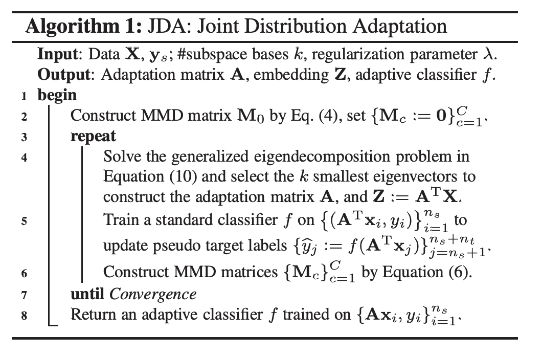
流程对应的伪代码如下

2.2. 学习策略

2.2.1. MMD距离

首先需要一个数学工具来表示两个分布的距离。这里用到了MMD距离。

最大均值差异（Maximum mean discrepancy，MMD），是一种用来度量两个不同但相关的分布的距离的方法，是一种常用于迁移学习中的Domain adaptation的核学习方法。

从名字中可以看出，这种方法主要是计算两个分布的均值（即期望）来反映两者的差异，原始计算公式也很简单 \[ \operatorname{MMD}[\mathcal{F}, p, q] =\sup _{f \in \mathcal{F}}\left(\mathbf{E}_{p}[f(x)]-\mathbf{E}_{q}[f(y)]\right) \] 其中，\(f\) 是从属于 \(\mathcal{F}\) 的函数，\(\sup(\cdot)\) 是一种作差运算

对应到当前问题，上式表示为 \[ \operatorname{MMD}[\mathcal{F}, \mathbf{A}^{\mathrm{T}} \mathbf{x}_{i}, \mathbf{A}^{\mathrm{T}} \mathbf{x}_{j}] =\left\|\frac{1}{n_{s}} \sum_{i=1}^{n_{s}} \mathbf{A}^{\mathrm{T}} \mathbf{x}_{i}-\frac{1}{n_{t}} \sum_{j=n_{s}+1}^{n_{s}+n_{t}} \mathbf{A}^{\mathrm{T}} \mathbf{x}_{j}\right\|^{2} \] 其中，\(\mathbf{A}^{\mathrm{T}} \mathbf{x}_{i}\) 和 \(\mathbf{A}^{\mathrm{T}} \mathbf{x}_{j}\) 便是当前问题中两个从属于 \(\mathcal{F}\) 空间中的分布

为了后序计算便利，将上式转化为矩阵形式，下面直接给出推导过程，至于和其他距离优缺点问题后面有时间再补吧=-= \[ \begin{array}{l} \left\|\frac{1}{n_{s}} \sum_{i=1}^{n_{s}} \mathbf{A}^{\mathrm{T}} \mathbf{x}_{i}-\frac{1}{n_{t}} \sum_{j=n_{s}+1}^{n_{s}+n_{t}} \mathbf{A}^{\mathrm{T}} \mathbf{x}_{j}\right\|^{2}\\ =\left\|\frac{1}{n_{s}} \mathbf{A}^{\mathrm{T}}\left[\begin{array}{llll} \mathbf{x}_{1} & \mathbf{x}_{2} & \cdots & \mathbf{x}_{n_{s}} \end{array}\right]_{1 \times n_{s}}\left[\begin{array}{c}1 \\1 \\ \vdots \\ 1 \end{array}\right]_{n_{s} \times 1}-\frac{1}{n_{t}} \mathbf{A}^{\mathrm{T}}\left[\begin{array}{llll} \mathbf{x}_{1} & \mathbf{x}_{2} & \cdots & \mathbf{x}_{n_{t}} \end{array}\right]_{1 \times n_{t}}\left[\begin{array}{c} 1 \\ 1 \\ \vdots \\ 1 \end{array}\right]_{n_{t} \times 1}\right\|^{2}\\ =\operatorname{tr}\left(\frac{1}{n_{s}^{2}} \mathbf{A}^{\mathrm{T}} \mathbf{X}_{s} \mathbf{1}\left(\mathbf{A}^{\mathrm{T}} \mathbf{X}_{s} \mathbf{1}\right)^{\mathrm{T}}+\frac{1}{n_{t}^{2}} \mathbf{A}^{\mathrm{T}} \mathbf{X}_{t} \mathbf{1}\left(\mathbf{A}^{\mathrm{T}} \mathbf{X}_{t} \mathbf{1}\right)^{\mathrm{T}}-\frac{1}{n_{s} n_{t}} \mathbf{A}^{\mathrm{T}} \mathbf{X}_{s} \mathbf{1}\left(\mathbf{A}^{\mathrm{T}} \mathbf{X}_{t} \mathbf{1}\right)^{\mathrm{T}}-\frac{1}{n_{s} n_{t}} \mathbf{A}^{\mathrm{T}} \mathbf{X}_{t} \mathbf{1}\left(\mathbf{A}^{\mathrm{T}} \mathbf{X}_{s} \mathbf{1}\right)^{\mathrm{T}}\right)\\ =\operatorname{tr}\left(\frac{1}{n_{s}^{2}} \mathbf{A}^{\mathrm{T}} \mathbf{X}_{s} \mathbf{1} \mathbf{1}^{\mathrm{T}} \mathbf{X}_{s}^{\mathrm{T}} \mathbf{A}+\frac{1}{n_{t}^{2}} \mathbf{A}^{\mathrm{T}} \mathbf{X}_{t} \mathbf{1} \mathbf{1}^{\mathrm{T}} \mathbf{X}_{t}^{\mathrm{T}} \mathbf{A}-\frac{1}{n_{s} n_{t}} \mathbf{A}^{\mathrm{T}} \mathbf{X}_{s} \mathbf{1} \mathbf{1}^{\mathrm{T}} \mathbf{X}_{t}^{\mathrm{T}}-\frac{1}{n_{s} n_{t}} \mathbf{A}^{\mathrm{T}} \mathbf{X}_{t} \mathbf{1 1}^{\mathrm{T}} \mathbf{X}_{s}^{\mathrm{T}}\right)\\ =\operatorname{tr}\left[\mathbf{A}^{\mathrm{T}}\left(\frac{1}{n_{s}^{2}} \mathbf{1 1}^{\mathrm{T}} \mathbf{X}_{s}^{\mathrm{T}} \mathbf{X}_{s}+\frac{1}{n_{t}^{2}} \mathbf{1 1} \mathbf{X}_{t}^{\mathrm{T}} \mathbf{X}_{t}-\frac{1}{n_{s} n_{t}} \mathbf{1} \mathbf{1}^{\mathrm{T}} \mathbf{X}_{s}^{\mathrm{T}} \mathbf{X}_{t}-\frac{1}{n_{s} n_{t}} \mathbf{1 1}^{\mathrm{T}} \mathbf{X}_{t}^{\mathrm{T}} \mathbf{X}_{s}\right) \mathbf{A}\right]\\ =\operatorname{tr}\left(\mathbf{A}^{\mathrm{T}}\left[\begin{array}{ll} \mathbf{X}_{s} & \mathbf{X}_{t} \end{array}\right]\left[\begin{array}{cc} \frac{1}{n_{s}^{2}} \mathbf{1 1} & \frac{-1}{n_{s} n_{t}} \mathbf{1 1}^{\mathrm{T}} \\ \frac{-1}{n_{s} n_{t}} \mathbf{1 1}^{\mathrm{T}} & \frac{1}{n_{t}^{2}} \mathbf{1 1} \end{array}\right]\left[\begin{array}{l} \mathbf{X}_{s} \\ \mathbf{X}_{t} \end{array}\right] \mathbf{A}\right)\\ =\operatorname{tr}\left(\mathbf{A}^{\mathrm{T}} \mathbf{X} \mathbf{M} \mathbf{X}^{\mathrm{T}} \mathbf{A}\right) \end{array} \]

引入核技巧 \[ \begin{array}{l} \left\|\frac{1}{n_{s}} \sum_{i=1}^{n_{s}} \phi\left(\mathbf{x}_{i}\right)-\frac{1}{n_{t}} \sum_{j=1}^{n_{t}} \phi\left(\mathbf{x}_{j}\right)\right\|^{2}\\ =\operatorname{tr}\left(\left[\begin{array}{ll} \phi\left(\mathbf{x}_{s}\right) & \phi\left(\mathbf{x}_{t}\right) \end{array}\right]\left[\begin{array}{cc} \frac{1}{n_{s}^{2}} \mathbf{1 1}^{\mathrm{T}} & \frac{-1}{n_{s} n_{t}} \mathbf{1 1} \\ \frac{-1}{n_{s} n_{t}} \mathbf{1 1} & \frac{1}{n_{t}^{2}} \mathbf{1 1} \end{array}\right]\left[\begin{array}{l} \phi\left(\mathbf{x}_{s}\right) \\ \phi\left(\mathbf{x}_{t}\right) \end{array}\right]\right)\\ =\operatorname{tr}\left(\left[\begin{array}{c} \phi\left(\mathbf{x}_{s}\right) \\ \phi\left(\mathbf{x}_{t}\right) \end{array}\right]\left[\begin{array}{ll} \phi\left(\mathbf{x}_{s}\right) & \phi\left(\mathbf{x}_{t}\right) \end{array}\right]\left[\begin{array}{cc} \frac{1}{n_s^{2}} \mathbf{1 1} & \frac{-1}{n_{s}n_{t}} \mathbf{1 1} \\ \frac{-1}{n_{s} n_{t}} \mathbf{1 1} & \frac{1}{n_{t}^{2}} \mathbf{1 1} \end{array}\right]\right)\\ =\operatorname{tr}\left(\left[\begin{array}{ll} <\phi\left(\mathbf{x}_{s}\right), \phi\left(\mathbf{x}_{s}\right)> & <\phi\left(\mathbf{x}_{s}\right), \phi\left(\mathbf{x}_{t}\right)> \\ <\phi\left(\mathbf{x}_{t}\right), \phi\left(\mathbf{x}_{s}\right)> & <\phi\left(\mathbf{x}_{t}\right), \phi\left(\mathbf{x}_{t}\right)> \end{array}\right] \mathbf{M}\right)\\ =\operatorname{tr}\left(\left[\begin{array}{ll} K_{s, s} & K_{s, t} \\ K_{t, s} & K_{t, t} \end{array}\right] \mathbf{M}\right) \end{array} \] 其中 \[ (M)_{i j}=\left\{\begin{array}{cc} \frac{1}{n_{s} n_{s}}, & \mathbf{x}_{i}, \mathbf{x}_{j} \in \mathcal{D}_{s} \\ \frac{1}{n_{t} n_{t}}, & \mathbf{x}_{i}, \mathbf{x}_{j} \in \mathcal{D}_{t} \\ \frac{-1}{n_{s} n_{t}}, & \text { otherwise } \end{array}\right. \]

2.2.2. 边缘分布适配

现在有了MMD距离，边缘分布\(P(\mathbf{A}^{\mathrm{T}} \mathbf{x}_{s})\) 和 \(P(\mathbf{A}^{\mathrm{T}} \mathbf{x}_{t})\) 间的距离就很容易得出 \[ \begin{aligned} D(\mathbf{A}^{\mathrm{T}} \mathbf{x}_{i}, \mathbf{A}^{\mathrm{T}} \mathbf{x}_{j}) &= \left\|\frac{1}{n} \sum_{i=1}^{n} \mathbf{A}^{\mathrm{T}} \mathbf{x}_{i}-\frac{1}{m} \sum_{j=n+1}^{n+m} \mathbf{A}^{\mathrm{T}} \mathbf{x}_{j}\right\|_{\mathcal{H}}^{2} \\ &= \operatorname{tr}\left(\mathbf{A}^{\mathrm{T}} \mathbf{X} \mathbf{M}_{0} \mathbf{X}^{\mathrm{T}} \mathbf{A}\right) \end{aligned} \] 其中， \[ \left(\mathbf{M}_{0}\right)_{i j}=\left\{\begin{array}{ll} \frac{1}{n^{2}}, & \mathbf{x}_{i}, \mathbf{x}_{j} \in \mathcal{D}_{s} \\ \frac{1}{m^{2}}, & \mathbf{x}_{i}, \mathbf{x}_{j} \in \mathcal{D}_{t} \\ -\frac{1}{m n}, & \text { otherwise } \end{array}\right. \]

这一步和TCA的做法是类似的

TCA论文原文，后面有时间再补

2.2.3. 条件分布适配

条件分布 \(P(\mathbf{y}|T(\mathbf{x}))\) 是不能直接得出的，一般使用贝叶斯公式进行转换 \[ P(\mathbf{y}|T(\mathbf{x}_{s})) = \frac{P(\mathbf{y})P(T(\mathbf{x})|\mathbf{y})}{P(T(\mathbf{x}))} \] 其中，\(P(\mathbf{y})\) 是直接可求的，\(P(T(\mathbf{x}_{s}))\) 是可被忽略的，所以问题最终转化为求 \(P(T(\mathbf{x}_{s})|\mathbf{y}_s)\) 和 \(P(T(\mathbf{x}_{t})|\mathbf{y}_t)\) 间的距离

但由于目标域并没有标签，所以 \(P(T(\mathbf{x}_{t})|\mathbf{y}_t)\) 并不能直接得出。考虑到源域是有标签的，所以可以使用源域训练一个基分类器，然后使用基分类对目标域进行预测，便得到目标域的伪标签 \(\mathbf{y}'_t\)

至于为什么可以这样做，因为模型的最终目标是将源域和目标域投影到同一空间成为同一个分布，那适用于源域的分类器当然也适用于目标域。所以模型实际上是预先做了一个假设，认为两个数据域转换后已经是同一分布，只要后面证明两者的差异的确是很小的，那么一开始的假设就成立了。

\[ \begin{aligned} D(\mathbf{A}^{T} \mathbf{x}_{s}|\mathbf{y}_s,\mathbf{A}^{T} \mathbf{x}_{t}|\mathbf{y}'_t) &= \sum_{c=1}^{C} \left\|\frac{1}{n_{c}} \sum_{\mathbf{x}_{s_{i}} \in \mathcal{D}_{s}^{(c)}} \mathbf{A}^{T} \mathbf{x}_{s_{i}}-\frac{1}{m_{c}} \sum_{\mathbf{x}_{t_{i}} \in \mathcal{D}_{t}^{(c)}} \mathbf{A}^{T} \mathbf{x}_{t_{i}}\right\|_{\mathcal{H}}^{2} \\ &=\sum_{c=1}^{C} \operatorname{tr}\left(\mathbf{A}^{T} \mathbf{X} \mathbf{M}_{c} \mathbf{X}^{T} \mathbf{A}\right) \end{aligned} \]

其中， \[ \left(M_{c}\right)_{i j}=\left\{\begin{array}{ll} \frac{1}{n_{s}^{(c)} n_{s}^{(c)}}, & \mathbf{x}_{i}, \mathbf{x}_{j} \in \mathcal{D}_{s}^{(c)} \\ \frac{1}{n_{t}^{(c)} n_{t}^{(c)}}, & \mathbf{x}_{i}, \mathbf{x}_{j} \in \mathcal{D}_{t}^{(c)} \\ \frac{-1}{n_{s}^{(c)} n_{t}^{(c)}}, & \left\{\begin{array}{ll} \mathbf{x}_{i} \in \mathcal{D}_{s}^{(c)}, \mathbf{x}_{j} \in \mathcal{D}_{t}^{(c)} \\ \mathbf{x}_{j} \in \mathcal{D}_{s}^{(c)}, \mathbf{x}_{i} \in \mathcal{D}_{t}^{(c)} \end{array}\right. \\ 0, & \text { otherwise } \end{array}\right. \]

2.3. 学习算法

将上面的两个距离结合，便得到模型的目标函数 \[ \min \sum_{c=0}^{C} \operatorname{tr}\left(\mathbf{A}^{T} \mathbf{X} \mathbf{M}_{c} \mathbf{X}^{T} \mathbf{A}\right)+\lambda\|\mathbf{A}\|_{F}^{2} \] > 注：上式的c是从0开始的

为了保持变换前后数据的方差维持不变，所以还得加入限制条件 \[ \mathbf{A}^{T} \mathbf{X} \mathbf{H} \mathbf{X}^{T} \mathbf{A}=\mathbf{I} \] 其中，\(\mathbf{H}\) 是中心矩阵，\(\mathbf{I}\) 是单位矩阵

综上，便得到模型最终的目标函数 \[ \min \sum_{c=0}^{C} \operatorname{tr}\left(\mathbf{A}^{T} \mathbf{X} \mathbf{M}_{c} \mathbf{X}^{T} \mathbf{A}\right)+\lambda\|\mathbf{A}\|_{F}^{2} \\ \text { s.t. } \quad \mathbf{A}^{T} \mathbf{X} \mathbf{H} \mathbf{X}^{T} \mathbf{A}=\mathbf{I} \] 至于该公式的求解，看到最值约束问题，用拉格朗日就对了。具体的求解过程可以参考这篇笔记：分类算法-最大熵模型

最终得到的求解公式为 \[ \left(\mathbf{X} \sum_{c=0}^{C} \mathbf{M}_{c} \mathbf{X}^{T}+\lambda \mathbf{I}\right) \mathbf{A}=\mathbf{X} \mathbf{H} \mathbf{X}^{T} \mathbf{A} \Phi \] 其中，\(\Phi\) 为拉格朗日乘子

至于上面这个式子，是可以通过直接计算求解的，所以不需要进行数值计算，即反向传播迭代。