1. 通用属性
1.1. axis
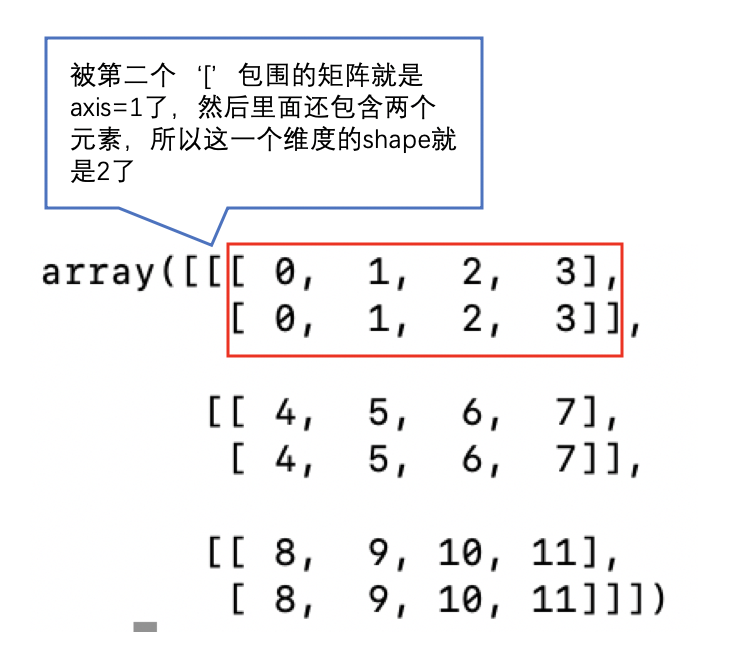
数组有多少个轴就是数组有多少个维度。
现在有一个数组arr.shape -> (1, 2, 3, 4),那么这是一个4维的数组,其中,axis=0表示第一维,其大小是1,表示有1个元素,axis=-1表示最后一维,即第四维,其大小是4,表示有4个元素。
一般是通过深度优先(即通过判断数矩阵符号 [ )来判断数组的axis和shape
另外,一般对数组处理的函数都有axis这个参数,如果不加特殊说明,这个参数一般默认为axis=None,这个参数下,会先把原数组压平成一维,然后再进行相应的操作,例如,a = np.sum(arr) -> a.shape -> (1, )
如果指定了axis参数,一般只改变指定的那个axis,其余的axis保持不变,例如,a = np.sum(arr, axis=1) -> a.shape -> (1, 1, 3, 4)
这给我们一个提示,如果我们进行数学运算或者数组操作的时候,有一个偷懒的技巧,那就是我们其实可以完全不用考虑我们要在哪一个axis进行运算,我们只需要知道哪一个axis会发生变化就可以了,例如,上面shape是(1, 2, 3, 4)的数组,我们想求和操作后得到一个(1, 1, 3, 4)的shape的数组,第二个维度的shape发生了变化,那就np.sum(arr, axis=1)就好了。
1.2. view
np中的view有点类似c++中的指针,所有的切片操作(高级索引返回的是copy)返回的都是view,一些函数返回的是view,
例如
>>> arr = np.array([[0, 1], [2, 3]])
>>> a = arr[:, 0]
>>> a[0] = 100
>>> a[0]
100
>>> arr[0][0]
100有个问题,例如,如果从一个大数组里面切片得到一个小数组,只要后续仍然存在对小数组引用,即使后面的操作中已经用不上原来的大数组了,但这个大数组仍然不会被Python垃圾处理机制处理释放内存,而且很多时候你并不确定后面对小数组的操作是否是独立,所以建议加上.copy()或者copy=True
1.3. broadcast
广播功能是numpy的一个很重要的功能,当两个维度不一样的数组进行运算时,会对低维的数组进行扩维后再进行运算,注意,这个低维向高维的扩维中,低维数组的维度必须和高维数组最后几维的维度一样
例如:
>>> a = np.zeros((2, 3, 4, 5))

# 这里运算其实是先把b扩展为shape为(2, 3, 4, 5)的数组,然后再进行对应维度相加
>>> b = 1
>>> a + b

# 这里和前面的原理是一样的,先把b扩展为shape为(2, 3, 4, 5)的数组,然后再进行对应维度相加
>>> b = np.zeros((4, 5))
>>> a + b

# b无法扩维,报广播错误
>>> b = np.zeros((3, 4))
>>> a + b
ValueError: operands could not be broadcast together with shapes (2,3,4,5) (3,4)
1.4. order
这是一个比较难搞的参数,这个参数是np与内存I/O的方法有关,是按照类C语言的规则还是按照FORTRAN类语言的规则。
order一般有四个参数‘K’, ‘A’, ‘C’, ‘F’,一般默认是'K'
“C”指的是用类C写的读/索引顺序的元素,最后一个维度变化最快,第一个维度变化最慢。以二维数组为例,简单来讲就是横着读,横着写,优先读/写一行。
“F”是指用FORTRAN类索引顺序读/写元素,最后一个维度变化最慢,第一个维度变化最快。竖着读,竖着写,优先读/写一列。注意,“C”和“F”选项不考虑底层数组的内存布局,只引用索引的顺序。
“A”选项所生成的数组的效果与原数组的数据存储方式有关,如果数据是按照FORTRAN存储的话,它的生成效果与”F“相同,否则与“C”相同。
"K"选项会自动返回一个与原数据最相似的order,一般就是"C"了
其如果对于内存读写没有太多的要求,这个参数跳过就好。后面提及这个参数的时候,也有给出一些例子。
2. 创建数组
2.1. 基于数据
2.1.1. np.array()
>>> np.array([[1, 2], [3, 4]])
array([[1, 2],
       [3, 4]])

# 输出数组的最低维度,如果输出维度比设定值小,就会对其进行扩维处理。
>>> np.array([1, 2, 3], ndmin=2)
array([[1, 2, 3]])
2.2. 基于形状
下列的方法都可以通过添加_like后缀,传入一个array_like参数,创建一个跟传入的array拥有相同的shape的数组,例如,arr.shape = (2,3) -> arr_ = np.zeros_like(arr) -> arr_.shape = (2,3)
下列的方法一般默认的返回类型是numpy.float64,所以如果想要一个整型的array,记得设置dtype!
2.2.1. np.zeros()
创建一个全是0的数组
>>> np.zeros((2, 1))
array([[ 0.],
       [ 0.]])

>>> np.zeros((2,), dtype=[('x', 'i4'), ('y', 'i4')]) # custom dtype
array([(0, 0), (0, 0)],
      dtype=[('x', '<i4'), ('y', '<i4')])
2.2.2. np.ones()
创建一个全是1的数组
>>> np.ones((2, 1))
array([[1.],
       [1.]])
2.2.3. np.empty()
创建一个随机初始化的数组
>>> np.empty([2, 2])
array([[ -9.74499359e+001,   6.69583040e-309],
       [  2.13182611e-314,   3.06959433e-309]])
2.2.4. np.full()
创建一个全是给定数值的数组
>>> np.full((2, 2), 10)
array([[10, 10],
       [10, 10]])
2.3. 特殊数组
2.3.1. np.eye()
返回一个二维数组,对角线上都为1,其他地方为零。
# 等价于 np.identity(2)
>>> np.eye(2)
array([[1., 0.],
       [0., 1.]])

>>> np.eye(3, k=1)
array([[0.,  1.,  0.],
       [0.,  0.,  1.],
       [0.,  0.,  0.]])
2.3.2. np.diag()
提取对角线或构造对角线数组
>>> arr
array([[0, 1, 2],
       [3, 4, 5],
       [6, 7, 8]])

>>> np.diag(arr)
array([0, 4, 8])
2.3.3. np.diagflat()
使用展平的输入作为对角线创建二维数组
np.diagflat([[1,2], [3,4]])
array([[1, 0, 0, 0],
       [0, 2, 0, 0],
       [0, 0, 3, 0],
       [0, 0, 0, 4]])
2.3.4. np.tri()
在给定对角线处及以下且在其他位置为零的数组
np.tril:数组的下三角
np.triu:数组的上三角
>>> np.tri(3, 5)
array([[1. 0. 0. 0. 0.]
 			[1. 1. 0. 0. 0.]
 			[1. 1. 1. 0. 0.]])
2.4. 区间
2.4.1. np.arange()
>>> np.arange(0, 1, 0.2)
array([0.  0.2 0.4 0.6 0.8])
2.4.2. np.linsapace()
>>> np.linspace(0, 1, 5)
array([0.   0.25 0.5  0.75 1.  ])
2.4.3. np.mgid
返回一个密集的多维“ meshgrid”
>>> np.mgrid[0:5,0:5]
array([[[0, 0, 0, 0, 0],
        [1, 1, 1, 1, 1],
        [2, 2, 2, 2, 2],
        [3, 3, 3, 3, 3],
        [4, 4, 4, 4, 4]],
       [[0, 1, 2, 3, 4],
        [0, 1, 2, 3, 4],
        [0, 1, 2, 3, 4],
        [0, 1, 2, 3, 4],
        [0, 1, 2, 3, 4]]])

>>> np.mgrid[-1:1:5j]
array([-1. , -0.5,  0. ,  0.5,  1. ])
2.4.4. np.ogrid
返回一个开放的多维“ meshgrid”
>>>> np.ogrid[0:5,0:5]
[array([[0],
        [1],
        [2],
        [3],
        [4]]), array([[0, 1, 2, 3, 4]])]

>>> np.ogrid[-1:1:5j]
array([-1. , -0.5,  0. ,  0.5,  1. ])
2.4.5. np.meshgrid()
主要是用来生成二维或三维图像
# x.shape -> (i, ); y.shape -> (j, )
# xv.shape -> (i, j); yv.shape -> (i, j)
>>> nx, ny = (3, 2)
>>> x = np.linspace(0, 1, nx)
>>> y = np.linspace(0, 1, ny)
>>> xv, yv = np.meshgrid(x, y)
>>> xv
array([[0. , 0.5, 1. ],
       [0. , 0.5, 1. ]])
>>> yv
array([[0., 0., 0.],
[1., 1., 1.]])举个例子:现在有一个图像的二维数组,其中每个像素的颜色函数为\(color(x, y) = sin(x) + cos(y)\),这个这个color数组可以用以下两种方法得到,效果是一样的,但后者消耗的时间更少
x, y = np.arange(300), np.arange(400)

# function 1
color = np.zeros((400, 300))
for i, x_ in enumerate(x):
    for j, y_ in enumerate(y):
        color[j, i] = np.sin(x_) + np.cos(y_)

# function 2
xv, yv = np.meshgrid(x, y)
color = np.sin(xv) + np.cos(yv)
2.5. 随机数组
一般都是用到np.random模块,这个模块相当重要
可以使用np.random.seed(n)来设置随机种子,这个设置时全局性的,意味着所有基于numpy的package,像sklearn、tensorflow等,只要设置了这个参数,每次的运行的结果都是固定的。
2.5.1. np.random.rand()
返回一个值在 [0, 1) 中均匀分布的随机样本
np.random.random_sample() 的作用这个方法是一样的
>>> np.random.rand(3)
array([0.96217732, 0.89279896, 0.75901262])

>>> np.random.rand(3,2)
array([[0.94300483, 0.00312197],
       [0.33184266, 0.9608146 ],
       [0.4771137 , 0.40549742]])
2.5.2. np.random.randn()
返回一个基于标准正态分布的随机数组
标准正态分布曲线下面积分布规律:
在-1.96~+1.96范围内曲线下的面积等于0.9500(即取值在这个范围的概率为95%),在-2.58~+2.58范围内曲线下面积为0.9900(即取值在这个范围的概率为99%)
如果要获取一般正态分布\(N(\mu,\sigma ^ {2})\),可以使用sigma * np.random.randn() + mu 或者 np.random.normal(mu, sigma, size)
np.random.standard_normal()、numpy.random.random()、numpy.random.ranf()、numpy.random.sample() 这些方法的作用和np.random.randn()是一样的
>>> np.random.randn(2)
array([1.76405235, 0.40015721])

>>> np.random.randn(2, 3)
array([[ 1.86755799, -0.97727788,  0.95008842],
[-0.15135721, -0.10321885, 0.4105985 ]])创建其他类型的随机分布数组可以查看这里
2.5.3. np.random.randint()
返回在给定的区间 [low, high) 内均匀分布的整数随机样本
如果要返回一个在 [a, b) 区间N等分取值,可以使用 a + (b - a) * (np.random.random_integers(N) - 1) / (N - 1.)
# 如果high=None,则数值区间在[0, low)
>>> np.random.randint(2, size=10)
array([1, 0, 0, 0, 1, 1, 0, 0, 1, 0])

>>> np.random.randint(5, size=(2, 4))
array([[4, 0, 2, 1],
       [3, 2, 2, 0]])

# 生成三个整数,分别在[1, 3), [1, 5), [1, 10)之间
>>> np.random.randint(1, [3, 5, 10])
array([2, 2, 9])

>>> np.random.randint([1, 3, 5, 7], [[10], [20]])
array([[ 8,  6,  9,  7],
       [ 1, 16,  9, 12]])
2.5.4. np.random.choice()
从给定条件随机抽取元素
# a是int类型,从[0, 5)区间内抽取整数
# 仅支持一维的array-like类型,则从给定的元素中随机抽取
>>> np.random.choice(5, 3)
array([0, 3, 4])
>>> np.random.choice([1,2,3], 3)
array([3, 1, 1])

# 不重复抽取数据
# 相当于 np.random.permutation(np.arange(5))[:3]
>>> np.random.choice(5, 3, replace=False)
array([3,1,0])

# 规定每个数值抽取概率
>>> np.random.choice(5, 3, p=[0.1, 0, 0.3, 0.6, 0])
array([3, 3, 0])
2.5.5. np.shuffle()
随机打乱数组,注意这个打乱是在原数组的基础上打乱,而且也不是按维度打乱,返回的是None
np.random.permutation(x) 的功能和 np.shuffle(x) 的功能类似,但前者不是在原数组上打乱
>>> arr = np.arange(9).reshape((3, 3))
>>> np.random.shuffle(arr)
>>> arr
array([[3, 4, 5],
       [6, 7, 8],
       [0, 1, 2]])
2.6. 矩阵
2.6.1. np.mat()
矩阵主要用于与 scipy.sparse 进行交互,矩阵与矩阵间的运算都是线性代数层面的运算,例如,arrA*arrB 是对应位置相乘,而 matA*matB 是线性代数的乘法,两者的结果是不一样的。
scipy.sparse是一个创建稀疏矩阵的模块,使用方法如下>>> arr = np.zeros((2, 3)) >>> arr[0, 1] = 1 >>> arr array([[0., 1., 0.], [0., 0., 0.]]) >>> from scipy import sparse >>> sp = sparse.csr_matrix(arr) # 创建稀疏矩阵 >>> sp <2x3 sparse matrix of type '<class 'numpy.float64'>' with 1 stored elements in Compressed Sparse Row format> >>> print(sp) (0, 1) 1.0 >>> sp.toarray() array([[0., 1., 0.], [0., 0., 0.]]) >>> print(sp + sp) # 注意这里进行的是矩阵的运算,不是数组的运算,做乘法的时候要注意!!! (0, 1) 2.0
官方建议不要使用矩阵,因为一般函数返回的数据类型是adnarray,使用矩阵会使得矩阵和数组间的处理变得很麻烦,而且这个模块在以后的更新中会被移除。
>>> np.mat([1,2,3])
matrix([[1, 2, 3]])
2.7. 掩码数组
2.7.1. np.ma.masked_array()
一般用于屏蔽无效数据,掩码数组是np.ndarray的子类,所以普通的数组可以用的方法,掩码数组也可以用。
>>> ma = np.ma.masked_array([1,2,3,4,5], mask=[0, 0, 0, 1, 0])
>>> ma
masked_array(data=[1, 2, 3, --, 5],
             mask=[False, False, False,  True, False],
       fill_value=999999)

>>> ma.sum()
11

# 重新设置掩码
# 方法一
>>> ma[0] = np.ma.masked
>>> ma[0]
masked
>>> ma
masked_array(data=[--, 2, 3, --, 5],
             mask=[ True, False, False,  True, False],
       fill_value=999999)

# 方法二
>>> ma.mask = [0,0,0,0,1]
>>> ma
masked_array(data=[1, 2, 3, 4, --],
             mask=[False, False, False, False,  True],
       fill_value=999999)
3. 数组变换
3.1. 数组维度变化
下列方法举例用到的数组arr,如无特殊说明,都是基于下面这个数组
>>> arr = np.arange(12).reshape((3,4))
>>> arr
array([[ 0,  1,  2,  3],
       [ 4,  5,  6,  7],
       [ 8,  9, 10, 11]])
3.1.1. arr.flatten()
将原数组压平为一个一维的数组
arr.ravel() 和arr.flatten()方法功能上一样的,但前者返回的是view,后者返回的是copy,为了避免麻烦,一般都使用arr.flatten()
# before: shape -> (3, 4)
# after: shape -> (12,)
>>> arr.flatten()
array([ 0,  1,  2,  3,  4,  5,  6,  7,  8,  9, 10, 11])

# order='C'可以理解为纵向按维度从高到低压平
# order='F'可以理解为横向按维度从低到高压平
# 一般我会使用 arr.T.flatten(),表现效果是一样的
>>> arr.flatten(order='F')
array([ 0,  4,  8,  1,  5,  9,  2,  6, 10,  3,  7, 11])
3.1.2. arr.squeeze()
这也是一个把数组压平的方法,但他只能压平shape为1的axis
>>> x.shape
(1, 2, 1, 3)
>>> x.squeeze().shape
(2, 3)
>>> x.squeeze(axis=0).shape
(2, 1, 3)
3.1.3. arr.reshape()
在不更改数据的情况下为数组赋予新的形状
arr.resize() 是在原数组的基础上改变数组的形状
# -1代表不指定维度,这个数值由后面的维度计算出来,-1只能出现一次
# before: shape -> (3, 4)
# after: shape -> (4, 3)
>>> arr.reshape((-1, 3))
array([[ 0,  1,  2],
       [ 3,  4,  5],
       [ 6,  7,  8],
       [ 9, 10, 11]])

# order='C'可以理解为纵向按维度从高到低压平后再reshape
# order='F'可以理解为横向按维度从低到高压平后再reshape
>>> arr.reshape((-1, 3), order='F')
array([[ 0,  5, 10],
       [ 4,  9,  3],
       [ 8,  2,  7],
       [ 1,  6, 11]])
3.1.4. arr.transpose()
重新分配维度的shape
arr.T 等价于a.transpose((n, n-1, ..., 1, 0))
# 这个函数的意思是原来维度axis的顺序是[0, 1],然后按照维度axis顺序为[1, 0]重新排列数组
# before: shape -> (3, 4)
# after: shape -> (4, 3)
>>> arr.transpose((1, 0))
array([[ 0,  4,  8],
       [ 1,  5,  9],
       [ 2,  6, 10],
       [ 3,  7, 11]])
3.1.5. np.rot90()
数组逆时针旋转90度
# before: shape -> (3, 4)
# after: shape -> (4, 3)
>>> np.rot90(arr)
array([[ 3,  7, 11],
       [ 2,  6, 10],
       [ 1,  5,  9],
       [ 0,  4,  8]])
3.1.6. np.expand_dims()
把原数组扩展一维
# before: shape -> (3, 4)
# after: shape -> (1, 3, 4)
# 相当于 arr[np.newaxis, :, :] or arr[None, :, :]
>>> np.expand_dims(arr, axis=0)
array([[[ 0,  1,  2,  3],
        [ 4,  5,  6,  7],
        [ 8,  9, 10, 11]]])

# before: shape -> (3, 4)
# after: shape -> (1, 3, 4, 1)
# 相当于 arr[np.newaxis, :, :, np.newaxis] or arr[None, :, :, None]
>>> np.expand_dims(arr, axis=(0, -1))
array([[[[ 0],
         [ 1],
         [ 2],
         [ 3]],

        [[ 4],
         [ 5],
         [ 6],
         [ 7]],

        [[ 8],
         [ 9],
         [10],
         [11]]]])
3.1.7. np.pad()
返回一个填充的数组
# after pad -> shape -> (2 + 5 + 3, )
>>> a = [1, 2, 3, 4, 5]
>>> np.pad(a, (2, 3), constant_values=(0, 1))
array([0, 0, 1, 2, 3, 4, 5, 1, 1, 1])

# after pad -> shape -> (2 + 3 + 3, 2 + 4 + 3)
>>> np.pad(arr, (2, 3), constant_values=(0, 1))
array([[ 0,  0,  0,  0,  0,  0,  1,  1,  1],
       [ 0,  0,  0,  0,  0,  0,  1,  1,  1],
       [ 0,  0,  0,  1,  2,  3,  1,  1,  1],
       [ 0,  0,  4,  5,  6,  7,  1,  1,  1],
       [ 0,  0,  8,  9, 10, 11,  1,  1,  1],
       [ 0,  0,  1,  1,  1,  1,  1,  1,  1],
       [ 0,  0,  1,  1,  1,  1,  1,  1,  1],
       [ 0,  0,  1,  1,  1,  1,  1,  1,  1]])

# after pad -> shape -> (1 + 3 + 2, 3 + 4 + 4)
>>> np.pad(arr, ((1, 2), (3, 4)), constant_values=(0, 1))
array([[ 0,  0,  0,  0,  0,  0,  0,  1,  1,  1,  1],
       [ 0,  0,  0,  0,  1,  2,  3,  1,  1,  1,  1],
       [ 0,  0,  0,  4,  5,  6,  7,  1,  1,  1,  1],
       [ 0,  0,  0,  8,  9, 10, 11,  1,  1,  1,  1],
       [ 0,  0,  0,  1,  1,  1,  1,  1,  1,  1,  1],
[ 0, 0, 0, 1, 1, 1, 1, 1, 1, 1, 1]])pad还有蛮多的参数,更多pad参数介绍可以参考这里
3.1.8. np.insert()
沿给定轴在给定索引之前插入值
# before: shape -> (3, 4)
# after: shape -> (3*4+2, )
# 如果不加axis参数,默认会先把数组压平成一维后再插入
>>> np.insert(arr, (2, 3), -1)
array([ 0,  1, -1,  2, -1,  3,  4,  5,  6,  7,  8,  9, 10, 11])

# before: shape -> (3, 4)
# after: shape -> (3, 4+2)
>>> np.insert(arr, (2, 3), -1, axis=1)
array([[ 0,  1, -1,  2, -1,  3],
       [ 4,  5, -1,  6, -1,  7],
       [ 8,  9, -1, 10, -1, 11]])
3.1.9. np.tile()
插入重复元素
# before: shape -> (3, 4)
# after: shape -> (3, 4*2)
>>> np.tile(arr, 2)
array([[ 0,  1,  2,  3,  0,  1,  2,  3],
       [ 4,  5,  6,  7,  4,  5,  6,  7],
       [ 8,  9, 10, 11,  8,  9, 10, 11]])

# before: shape -> (3, 4)
# after: shape -> (1*2, 3, 4)
# 这里会先把原数组升维,再复制
>>> np.tile(arr, (2, 1, 1))
array([[[ 0,  1,  2,  3],
        [ 4,  5,  6,  7],
        [ 8,  9, 10, 11]],

       [[ 0,  1,  2,  3],
        [ 4,  5,  6,  7],
        [ 8,  9, 10, 11]]])
3.1.10. np.repeat()
这也是一个插入重复元素的方法。
# before: shape -> (3, 4)
# after: shape -> (2*3*4, )
# 如果不加axis参数,默认会先把数组压平成一维后再复制
>>> np.repeat(arr, 2)
array([ 0,  0,  1,  1,  2,  2,  3,  3,  4,  4,  5,  5,  6,  6,  7,  7,  8,
        8,  9,  9, 10, 10, 11, 11])

# before: shape -> (3, 4)
# after: shape -> (3, 4*2)
# 对比 np.tile(arr, 2)
>>> np.repeat(arr, 2, axis=1)
array([[ 0,  0,  1,  1,  2,  2,  3,  3],
       [ 4,  4,  5,  5,  6,  6,  7,  7],
       [ 8,  8,  9,  9, 10, 10, 11, 11]])
3.2. 数组重排
3.2.1. np.flip()
数组轴对称
flip(m, 0) is equivalent to flipud(m).
flip(m, 1) is equivalent to fliplr(m).
flip(m, n) corresponds to m[...,::-1,...] with ::-1 at position n.
flip(m) corresponds to m[::-1,::-1,...,::-1] with ::-1 at all positions.
flip(m, (0, 1)) corresponds to m[::-1,::-1,...] with ::-1 at position 0 and position 1.
# axis=None,按原点对称
>>> np.flip(arr)
array([[11, 10,  9,  8],
       [ 7,  6,  5,  4],
       [ 3,  2,  1,  0]])

>>> np.flip(arr, 0)
array([[ 8,  9, 10, 11],
       [ 4,  5,  6,  7],
       [ 0,  1,  2,  3]])
3.2.2. np.roll()
数组旋转,这里的旋转是数组内元素进行旋转,数组形状不变
>>> np.roll(arr, 1)
array([[11,  0,  1,  2],
       [ 3,  4,  5,  6],
       [ 7,  8,  9, 10]])

>>> np.roll(arr, 1, axis=0)
array([[ 8,  9, 10, 11],
       [ 0,  1,  2,  3],
       [ 4,  5,  6,  7]])
3.3. 数组合并
3.3.1. np.stack()
沿新轴连接一系列数组。
合并的数组必须具有相同的shape
例如,现在有两个array需要合并,arr0、arr1,且 arr0.shape -> (1, 2, 3)、 arr1.shape -> (1, 2, 3),axis=0时,合并后的 shape -> (1*2, 1, 2, 3) -> (2, 1, 2, 3)
# each arr.shape -> (3, 4)
# after concatenate -> (1*2, 3, 4)
>>> arrs = [arr for _ in range(2)]
>>> np.stack(arrs)
array([[[ 0,  1,  2,  3],
        [ 4,  5,  6,  7],
        [ 8,  9, 10, 11]],

       [[ 0,  1,  2,  3],
        [ 4,  5,  6,  7],
        [ 8,  9, 10, 11]]])
3.3.2. np.concatenate()
沿现有轴连接一系列数组
合并的数组必须具有相同的axis,且除连接的axis外的其他维度必须具有相同的shape
例如,现在有两个array需要合并,arr0、arr1,且 arr0.shape -> (1, 2, 3)、 arr1.shape -> (2, 2, 3),axis=0时,合并后的 shape -> (1+2, 2, 3) -> (3, 2, 3)
这里有一个让人迷惑的地方:
np.vstack() 或 np.r_[] 和np.concatenate(axis=0)的结果相同;
np.hstack() 和np.concatenate(axis=1)的结果相同;
np.dstack() 或 np.c_[] 和np.concatenate(axis=-1)的结果相同。
# each arr.shape -> (3, 4)
# after concatenate -> (3+3, 4)
>>> arrs = [arr for _ in range(2)]
>>> np.concatenate(arrs)
array([[ 0,  1,  2,  3],
       [ 4,  5,  6,  7],
       [ 8,  9, 10, 11],
       [ 0,  1,  2,  3],
       [ 4,  5,  6,  7],
       [ 8,  9, 10, 11]])

# 这里又一个让人迷惑的地方,np.c_可以合并一维数组,np.concatenate(axis=1)则不可以
>>> np.concatenate([np.array([1,2,3]), np.array([4,5,6])], axis=1)
Traceback (most recent call last):
  File "<stdin>", line 1, in <module>
  File "<__array_function__ internals>", line 6, in concatenate
numpy.AxisError: axis 1 is out of bounds for array of dimension 1
>>> np.c_[np.array([1,2,3]), np.array([4,5,6])]
array([[1, 4],
       [2, 5],
       [3, 6]])
3.3.3. np.block()
从块的嵌套列表中组装一个nd数组。理解为拼积木就可以了
# each arr.shape -> (3, 4)
# after block -> (3+3, 4+4)
>>> arrs = [[arr, arr],
...        [arr, arr]]
>>> np.block(arrs)
array([[ 0,  1,  2,  3,  0,  1,  2,  3],
       [ 4,  5,  6,  7,  4,  5,  6,  7],
       [ 8,  9, 10, 11,  8,  9, 10, 11],
       [ 0,  1,  2,  3,  0,  1,  2,  3],
       [ 4,  5,  6,  7,  4,  5,  6,  7],
       [ 8,  9, 10, 11,  8,  9, 10, 11]])
3.3.4. np.append()
将值附加到数组的末尾
# before: shape -> (3, 4)
# after: shape -> (3*4+3*4, )
# 如果不加axis参数,默认会先把数组压平成一维后再拼接
>>> np.append(arr, arr)
array([ 0,  1,  2,  3,  4,  5,  6,  7,  8,  9, 10, 11,  0,  1,  2,  3,  4,
        5,  6,  7,  8,  9, 10, 11])

# before: shape -> (3, 4)
# after: shape -> (3, 4+4)
>>> np.append(arr, arr, axis=1)
array([[ 0,  1,  2,  3,  0,  1,  2,  3],
       [ 4,  5,  6,  7,  4,  5,  6,  7],
       [ 8,  9, 10, 11,  8,  9, 10, 11]])
3.4. 数组拆分
3.4.1. np.split()
将数组拆分为多个子数组,返回的是view
np.vsplit(): 相当于np.split(axis=0)
np.hsplit(): 相当于np.split(axis=1)
np.dsplit(): 相当于np.split(axis=2)
# before arr.shape -> (3, 4)
# 把原数组按axis=0的维度,平均分成了3份,即[(1, 4), (1, 4), (1, 4)]
>>> np.split(arr, 3)
[array([[0, 1, 2, 3]]), array([[4, 5, 6, 7]]), array([[ 8,  9, 10, 11]])]

# 把原数组按axis=0的维度,分成大小为1、2、3的3份,后面不够的返回0就好了,即[(1, 4), (2, 4), (0, 4)]
>>> np.split(arr, [1, 2, 3])
[array([[0, 1, 2, 3]]), array([[4, 5, 6, 7]]), array([[ 8,  9, 10, 11]]), array([], shape=(0, 4), dtype=int64)]
3.5. 类型转换
3.5.1. arr.astype()
>>> arr = np.array([1, 2, 2.5])
>>> arr.astype(int)
array([1, 2, 2])
>>> arr.astype(str)
array(['1.0', '2.0', '2.5'], dtype='<U32')
4. 常用数组运算
4.1. 简单数学运算
numpy内置的数学函数实在太多了,这里就不一一列举了,具体的可以查阅这里
4.2. 线性代数运算
4.2.1. 矩阵乘法
对应位置相乘:arrA * arrB, np.multiply(arrA, arrB)
线性代数的矩阵乘法:arrA @ arrB, np.dot(arrA, arrB), np.matmul(arrA, arrB), matA * matB(尽量少用matrix这种形式)
>>> arrA = np.array([[1, 2], [2, 3]])
>>> arrB = np.array([[2, 2], [2, 2]])

>>> arrA * arrB
array([[2, 4],
       [4, 6]])

>>> arrA @ arrB	# 只适用于Python3.5以上的版本
array([[ 6,  6],
       [10, 10]])
4.2.2. np.linalg模块
这是numpy内置的线性代数模块,里面集合了很多线性代数的计算方法,具体可以查阅这里
4.3. 集合运算
# 差集
>>> np.setdiff1d([1, 3, 4, 3], [3, 1, 2, 1])
array([4])

# 交集
>>> np.intersect1d([1, 3, 4, 3], [3, 1, 2, 1])
array([1, 3])

# 并集
>>> np.union1d([1, 3, 4, 3], [3, 1, 2, 1])
array([1, 2, 3, 4])

# 异或
>>> np.setxor1d([1, 3, 4, 3], [3, 1, 2, 1])
array([2, 4])
4.4. 逻辑运算
>>> x = np.arange(5)

# 逻辑与
>>> np.logical_and(x>1, x<4)
array([False, False,  True,  True, False])

# 逻辑或
>>> np.logical_or(x>1, x<4)
array([ True,  True,  True,  True,  True])

# 逻辑非
>>> np.logical_not(x>1, x<4)
array([ True,  True, False, False, False])

# 逻辑异或
>>> np.logical_xor(x>1, x<4)
array([ True,  True, False, False,  True])
4.5. 排序,搜索
4.5.1. np.argsort()
返回将对数组进行从小到大排序的索引
类似的方法还有np.argmax() 和 np.argmin(),分别返回最大值和最小值的索引,这两个方法如果不设置axis,对二维以上的数组求索引时,返回的是一个int
>>> arr = np.random.randint(10, size=(3,4),)
>>> arr
array([[5, 1, 3, 3],
       [6, 5, 3, 2],
       [6, 8, 7, 3]])

>>> np.argsort(arr)
array([[1, 2, 3, 0],
       [3, 2, 1, 0],
       [3, 0, 2, 1]])

>>> np.argmax(arr)
9

>>> np.argmax(arr, axis=0)
array([1, 2, 2, 0])
5. 保存/读取
5.1. 保存
# 目录下生成test.npy文件,这个默认是调用pickle模块保存的
>>> np.save('test', arr)

# 目录下生成test.pyz文件,这是一个压缩后的二进制文件
>>> np.savez('test', arr)

# 目录下生成test.txt文件,这个文件可以直接查看
>>> np.savetxt('test.txt', arr)
5.2. 读取
>>> arr = np.load('test.npy')
>>> arr = np.load('test.npz')

>>> arr = np.loadtxt('test.txt')